Regression Modelling with Geographic Coordinates
Motivation and Introduction
Previously, a dashboard was built to visualize Bixi trips between 2014 and 2021. As a bicycle rental company, daily operations likely include the movement of bicycles between stations, whether to improve bicycle availability at popular stations or to make space at fully docked stations. In an effort to improve this process of restocking or emptying bicycle docking stations, a regression model was built and trained using the location of stations to predict how many trips start from each station on an annual basis.
The foundation of this model was based on the assumption that the location of a bicycle station affects how busy a station will be, and thus how much effort is needed for restocking or emptying. Furthermore, an assumption was made that although the annual number of trips changes, the percentage of annual trips for each station remains constant throughout the years, thus avoiding the need to use time-series models.
In the final random forest regression model, using RBF Kernel, each station’s latitude and longitude were converted to similarity measures to each of the 25 cluster centers identified through KMeans clustering. These similarity measures were used to predict the percentage of annual trips that start from each station. An intuitive understanding would be how locations are identified to be important based on its proximity to other landmarks.
The final model was tested to have a root mean square error 0.05608% percentage of annual trips, with a 95% confidence interval of 0.04770% and 0.06336%. These results indicate that the model only works well for stations with larger percentage of annual trips (>33% percentile). However, at an annual level, the final model’s predictions were within 0.1 million trips for all years except 2021. This suggests that the model has not “learned” the one time effects of Covid-19, and, that the errors for stations below the 33% percentile of annual trips were insignificant compared to the annual trips for busier stations.
Overview of Setup
Docker Environments
To replicate the environment used to perform this analysis:
- Fork the Github repository on a local machine with Docker and Docker-compose installed.
- Run below line in Terminal within the file directory of the repository
# Run below line in terminal within the folder that contains the forked repo
docker-compose -f dev_setup.yaml up
Instructions on how to access Jupyter will be generated in the Terminal. Detailed installation documentation can be found within the README of the repository.
Import Packages and Define Functions
The models and modelling pipelines were built from the Scikit-learn package.
# For general data processing
import numpy as np
import pandas as pd
import math
import time

# Custom functions for measuring time of queries and to print lists
from notebook_functions.timer import print_time
from notebook_functions.print import print_list

# Packages for data visualization
import matplotlib.pyplot as plt
from pandas.plotting import scatter_matrix
import seaborn as sns
from adjustText import adjust_text # For fine tuning position of text above points in scatterplot
import plotly.express as px

# For the engine that connects Python and MySQL
import sqlalchemy

# For building custom sklearn classes
from sklearn.base import BaseEstimator, TransformerMixin

# For data preprocessing and feature engineering
from sklearn.model_selection import train_test_split
from sklearn.compose import ColumnTransformer
from sklearn.pipeline import Pipeline, make_pipeline
from sklearn.impute import SimpleImputer
from sklearn.preprocessing import StandardScaler
from sklearn.cluster import KMeans
from sklearn.metrics.pairwise import rbf_kernel

# Models for testing
from sklearn.linear_model import LinearRegression
from sklearn.tree import DecisionTreeRegressor
from sklearn.ensemble import RandomForestRegressor
from sklearn.svm import SVR

# Model hyperparameter tuning and performance evaluation
from sklearn.metrics import mean_squared_error
from sklearn.model_selection import GridSearchCV
from scipy import stats

# For saving the model
import joblib
Import Data From MySQL
A SQLAlchemy engine was created and used to import data from MySQL into the Jupyter notebook. Ideally, the dotenv packaged would be used to load hidden credentials for access to MySQL. However, since this database is only available locally, the defaults were inputted plainly in engine creation.
# Create the connection engine to MySQL database called 'velocipede'
engine = sqlalchemy.create_engine(
    "mysql+mysqldb://root:rootroot@sql:3306/velocipede"
)
The below SQL query was used to transform and extract the number of rides starting at each station for each year along with station details such as station latitude and longitude. A join table, jt_rides_stations, was used given the rides table and stations table have a many to many relationship. Explanations are in included as comments in the SQL query below.
# SQL statement that gathers the number of rides per station per year along with station details
sql_stmt = """
# A CTE counting the number of rides per station per year
WITH a AS (
SELECT
    COUNT(ride_id) AS rides,
    YEAR(CONVERT_TZ(start_dt_utc,"+00:00","-04:00")) AS year,
    start_stn_code,
    data_source
FROM
    rides
WHERE
    company = "Bixi"
GROUP BY
    year,
    start_stn_code,
    data_source
)

# Main SQL statement that adds station details to the CTE using join table
SELECT
    SUM(a.rides) AS rides,
    a.year,
    a.start_stn_code,
    c.stn_name,
    c.stn_lat,
    c.stn_lon
FROM
    a

# left join #1 to join-table between rides and stations tables
LEFT JOIN
    jt_rides_stations AS b
ON
    a.data_source = b.ride_files

# left join #2 to stations table
LEFT JOIN
    stations AS c
ON
    b.station_files = c.data_source
    AND a.start_stn_code = c.stn_code
GROUP BY
    a.year,
    a.start_stn_code,
    c.stn_name,
    c.stn_lat,
    c.stn_lon
"""
# Establish MySQL connection through engine then run SQL query
with print_time():
    with engine.connect() as conn:
        df = pd.read_sql(
            sqlalchemy.text(sql_stmt),
            con = conn
        )
Time taken: 468.9603 seconds.
The query was observed to take more than 5 minutes to execute on the local machine as it involves 40.9 million rows of data. This demonstrates MySQL’s limitations in dealing with the scale of data, which can be overcome by using column oriented data file formats like Apache Parquet along with a PySpark cluster in future iterations.
The data resulting from the MySQL query was briefly examined before being saved as processed data to avoid re-running the SQL query again.
print(f"The data has {df.shape[0]} rows and {df.shape[1]} columns.")
print(f"The number of null values is {df.isna().sum().sum()}.")

# Visually examine the first few rows of data
df.head()
The data has 5394 rows and 6 columns.
The number of null values is 9.
| rides | year | start_stn_code | stn_name | stn_lat | stn_lon | |
|---|---|---|---|---|---|---|
| 0 | 4478.0 | 2021 | 10 | Métro Angrignon (Lamont / des Trinitaires) | 45.446910 | -73.603630 |
| 1 | 6871.0 | 2021 | 100 | 16e avenue / St-Joseph | 45.552870 | -73.565631 |
| 2 | 1093.0 | 2021 | 1000 | Parc Champdoré (Champdoré / de Lille) | 45.569176 | -73.636293 |
| 3 | 4469.0 | 2021 | 1002 | Vendôme / Sherbrooke | 45.475963 | -73.607234 |
| 4 | 3179.0 | 2021 | 1003 | Parc Tino-Rossi (18e avenue / Everett) | 45.564811 | -73.595804 |
# Save data to processed data folder for easy access
df.to_csv(f"../12_processed_data/{time.strftime('%Y%m%d-%H%M')}_rides_per_station_per_year.csv")
# Uncomment this line for loading the saved processed data
# df = pd.read_csv(f"../12_processed_data/20231003-1926_rides_per_station_per_year.csv", index_col = 0)
Exploratory Data Analysis (EDA)
Each row within the loaded data represents the number of Bixi bicycle rental trips(rides) that started at each station for each year. As a station’s location and name may remain constant or change slightly across the years, this means that a given station name may appear multiple times within the data. The data was explored for null values and any trends that maybe helpful for modelling later on.
Null values
# Select rows where any value in null
cond = df.isna().any(axis=1)
df.loc[cond]
| rides | year | start_stn_code | stn_name | stn_lat | stn_lon | |
|---|---|---|---|---|---|---|
| 3151 | 3800.0 | 2019 | 6034 | NaN | NaN | NaN |
| 3247 | 5941.0 | 2019 | 6708 | NaN | NaN | NaN |
| 5225 | 3.0 | 2019 | MTL-ECO5.1-01 | NaN | NaN | NaN |
Given only 3 stations had null station details in 2019, these 3 stations were dropped from analysis.
df = df.loc[~cond]

# Examine the data after dropping rows with null values
print(f"The data has {df.shape[0]} rows and {df.shape[1]} columns.")
print(f"The number of null values is {df.isna().sum().sum()}.")
The data has 5391 rows and 6 columns.
The number of null values is 0.
Rides by Year
Next, the numbers of Bixi trips were summed and plotted against years to identify annual trends.
# Reaggregate the data by year to count the number of rides per year
plot_df = df.groupby(
    by = ["year"]
).agg(
    rides = ("rides","sum")
)

# Use built in pandas plot method for quick plotting
plot_df.plot(
    kind = "bar",
    legend = None
)

# Tidy up plot
plt.xlabel("Year")
plt.ylabel("Number of Rides (millions)")
plt.title("Figure 1. Number of Bixi Rides by Year", y = -0.25)
sns.despine()
plt.show()
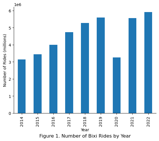
An annual increasing trend was observed, with the year 2020 being an exception most likely due to Covid-19 restrictions. To avoid training the model to fit special cases like Covid-19, the year 2020 was dropped from analysis. Furthermore, the year 2022 was also known to have incomplete data due to membership details being omitted starting 2022. As such, the years 2020 and 2022 were ommitted from analysis.
# Create condition to identify rows for 2020 and 2022
cond = df["year"].isin([2020,2022])

# Remove rows based on condition
df = df.loc[~cond]

# Examine the data after dropping rows with null values
print(f"The data has {df.shape[0]} rows and {df.shape[1]} columns.")
print(f"The number of null values is {df.isna().sum().sum()}.")
The data has 3926 rows and 6 columns.
The number of null values is 0.
Illogical Latitude and Longitudes
After checking annual rides, the latitude and longitudes of each station were checked to identify any erroneous station locations that are likely not representative of any location within the city of Montreal.
# Use built in function to examine distribution of columns
df[["stn_lat","stn_lon"]].describe()
| stn_lat | stn_lon | |
|---|---|---|
| count | 3926.000000 | 3926.000000 |
| mean | 45.507946 | -73.566578 |
| std | 0.743071 | 1.158884 |
| min | -1.000000 | -73.746873 |
| 25% | 45.501402 | -73.602610 |
| 50% | 45.523276 | -73.578050 |
| 75% | 45.539632 | -73.564776 |
| max | 45.651406 | -1.000000 |
Note that the minimum value for station latitude was -1, which is definitely not in Montreal.
# The rows where station latitude was less than 0 were identified and examined
cond = df.stn_lat < 0
display(df[cond])
| rides | year | start_stn_code | stn_name | stn_lat | stn_lon | |
|---|---|---|---|---|---|---|
| 704 | 9749.0 | 2021 | 856 | Smith / Peel | -1.0 | -1.0 |
As the this occured to only 1 row of data, the row in question was dropped.
df = df.loc[~cond]

# Examine the data after dropping rows with null values
print(f"The data has {df.shape[0]} rows and {df.shape[1]} columns.")
print(f"The number of null values is {df.isna().sum().sum()}.")
The data has 3925 rows and 6 columns.
The number of null values is 0.
Number of Stations per Year
Next the number of stations per year was examined. Given that the annual number of rides has increased steadily over the years in Figure 1, it was expected that the number of bicycle stations have also increased throughout the years to meet increasing demand.
# Reaggregate the data by year to count the number of rides per year
plot_df = df.groupby(
    by = ["year"]
).agg(
    stations = ("start_stn_code","nunique")
)

# Use built in pandas plot method |or quick plotting
plot_df.plot(
    kind = "bar",
    legend = None
)

plt.xlabel("Year")
plt.ylabel("Number of Stations")
plt.title("Figure 2. Number of Stations by Year", y = -0.25)
sns.despine()
plt.show()
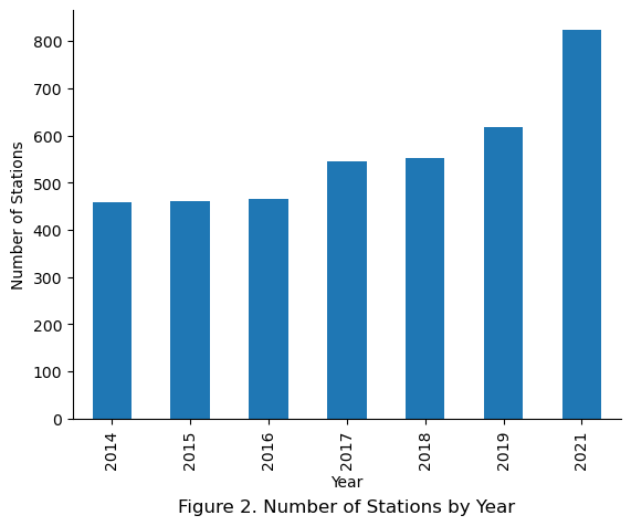
The number of stations were observed to increase as the years progress.
% of Trips by Station (Target Feature)
To avoid the need of employing time-series algorithms to deal with the increasing number of rides through the years, the popularity of a station was expressed as a percentage of total rides for the year, with the assumption that the relative popularity of a station’s location compared to other stations is roughly constant across the years. That way, the output of the model can be multiplied by the total number of rides expected for a given year to get the number of rides.
# Create new target feature: percentage of annual rides
df["pct_of_annual_rides"] = df["rides"] / df.groupby(by = ["year"])["rides"].transform("sum")
Then, the stations were ranked annually by descending number of trips starting at each station.
# Rank the stations by descending rides starting at each station for each year
df["annual_stn_rank"] = df.groupby(by = ["year"])["rides"].rank(method = "dense", ascending = False)
df["annual_stn_rank"] = df["annual_stn_rank"].astype(int)
Finally, the dataset was filtered and transformed to examine the percentage of annual rides held by the top 10 stations across the years regardless of station location.
# Filter for only the top 10 stations
cond = df["annual_stn_rank"] < 11

# Pivot the data so that the % of rides for the top 10 stations are compared across the years
rank_df = df.loc[cond].pivot(
    columns = "year",
    index = "annual_stn_rank",
    values = "pct_of_annual_rides"
)

# Visually examine the percentage of rides for the top 10 stations for each year
# Create and apply color map horizontally to dataframe
cm = sns.light_palette("blue", as_cmap = True)
s = rank_df.style.background_gradient(cmap = cm,axis = 1)
display(s)
| year | 2014 | 2015 | 2016 | 2017 | 2018 | 2019 | 2021 |
|---|---|---|---|---|---|---|---|
| annual_stn_rank | |||||||
| 1 | 0.014540 | 0.012901 | 0.010376 | 0.011894 | 0.010299 | 0.008547 | 0.008694 |
| 2 | 0.010599 | 0.009685 | 0.009940 | 0.008825 | 0.008339 | 0.007838 | 0.006525 |
| 3 | 0.010221 | 0.008819 | 0.009796 | 0.008549 | 0.008301 | 0.006743 | 0.006488 |
| 4 | 0.008999 | 0.008656 | 0.009719 | 0.008314 | 0.008117 | 0.006535 | 0.005788 |
| 5 | 0.008632 | 0.008437 | 0.008854 | 0.008030 | 0.007099 | 0.006289 | 0.005678 |
| 6 | 0.007795 | 0.007424 | 0.008046 | 0.007926 | 0.006965 | 0.005556 | 0.005677 |
| 7 | 0.007740 | 0.006860 | 0.007942 | 0.007866 | 0.006015 | 0.005354 | 0.005501 |
| 8 | 0.007199 | 0.006471 | 0.007371 | 0.006973 | 0.005993 | 0.005321 | 0.005356 |
| 9 | 0.007104 | 0.006456 | 0.006778 | 0.006428 | 0.005639 | 0.005300 | 0.005233 |
| 10 | 0.006951 | 0.006302 | 0.006418 | 0.006217 | 0.005481 | 0.005264 | 0.004693 |
Here, the assumption that the percentage of annual rides for each station being constant was observed to be roughly applicable for the years 2014 to 2018, with the years 2019 and beyond showing a deviation from the assumption. Specifically, in 2014 the top 1 station represented 1.45% of annual rides compared to only 0.85% in 2019.
# Plot the % of rides taken by the top 10 stations for each year
(rank_df.sum()*100).plot()

# Add in labels
plt.xlabel("Year")
plt.ylabel("% of annual rides for top 10 stations")
plt.title("Figure 3. Percentage of Annual Rides Represented by Top 10 Stations", y = -0.25)
sns.despine()
plt.show()
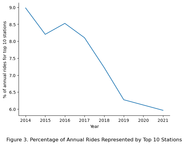
Taking the sum of the top 10 stations revealed that the percentage of annual rides represented by the top 10 stations reduces as the years go on, with the observed dilution likely due to more stations being introduced with each new year.
That being said, for the keeping the model simple in this analysis, the assumption that the percentage of annual per station remains constant was upheld with note for improvement in future iterations.
Station Location
A brief scatterplot of all station locations was visually examined to confirm that the stations do indeed represent a rough map of the city of Montreal.
# Create scatter plot of station location
df.plot(
    kind = "scatter",
    y = "stn_lat",
    x = "stn_lon",
    c = "cornflowerblue",
    alpha = 0.2
)

# tidy up chart
plt.xlabel(f"Station Longitude")
plt.ylabel(f"Station Latitude")
plt.title(f"Figure 4. Scatterplot of Bixi Stations", y = -0.25)
sns.despine()
plt.show()
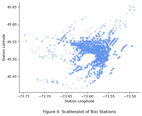
The opacity represents the density fo stations across the years. The dark blue areas represent the downtown core of Montreal while the blank patch centered at -73.60 and 45.50 represents Mount Royal, confirming that the data is indeed stations located within Montreal.
Correlations
As the station latitudes and longitudes will be preprocessed later using KMeans clustering and RBF Kernel, observed correlations should be taken with a grain of salt.
# Define columns for correlation checking
cols = ["pct_of_annual_rides","stn_lat","stn_lon"]

# Plot a scatterplot matrix for defined columns
scatter_matrix(df[cols],figsize = (12,8))
plt.title("Figure 5. Correlation Scatterplot Matrix", x = -0.5, y = -0.50)
plt.show()
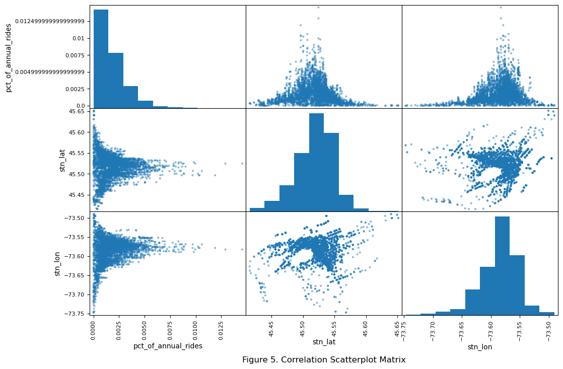
The top left histogram suggests a right skewed distribution of the target feature. Looking at the middle and right scatterplots in the top row suggest that stations in the city center of Montreal have higher percentage of annual rides.
Summary of Data Cleaning
| Data Cleaning Operation | Rows Removed | Rows Remaining |
|---|---|---|
| - | - | 5,394 |
| Drop null values | 3 | 5,391 |
| Remove 2020 and 2022 | 2,095 | 3,296 |
| Station latitude < 0 | 1 | 3,295 |
Data Preprocessing
Stratification
The target feature of prediction, pct_of_annual_rides, was observed to have a non-uniform, right skewed distribution. To ensure consistent target feature distribution across the test and training sets, the target feature, being continuous and numerical, was first converted into a categorical variable for stratification. As a balance between the number categories and the number of rows for each category, the data was split into 3 parts based onto their quantiles using the pd.cut method.
# Define target_feature or y
y = df["pct_of_annual_rides"]

# Define boundaries to cut up numerical target feature into categorical bins.
# 3 parts, so four boundaries
cat_bin_boundaries = [
    0,
    y.quantile(q=0.33).round(5),
    y.quantile(q=0.66).round(5),
    np.inf
]

# Define labels for each bin
cat_bin_labels = [
    "00 - 33% percentile",
    "34 - 66% percentile",
    "67 - 100% percentile"
]

# Categorize target feature based on defined boundaries and labels
df["pct_cat"] = pd.cut(
    y,
    bins = cat_bin_boundaries,
    labels = cat_bin_labels
)

# Plot a count of the categorized target feature
df["pct_cat"].value_counts().sort_index().plot.bar(rot = 0)
plt.ylabel("Number of data points")
plt.xlabel("Target Feature Categories")
plt.title(f"Figure 6. 'pct_of_annual_rides' categorized by Percentiles", y = -0.2)
sns.despine()
plt.show()
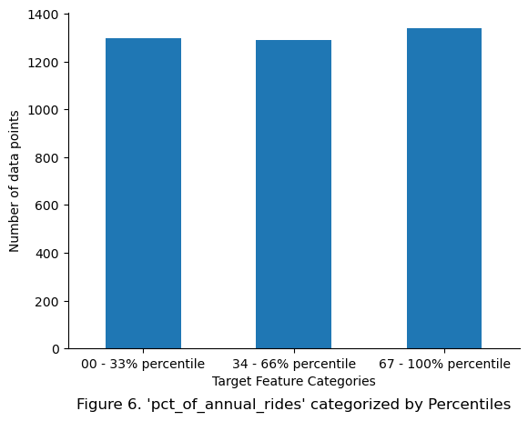
The figure demonstrates how pct_of_annual_rides was split into 3 even categories for stratification. For further visual verification, the original distribution of the target feature was mapped according to the 3 defined categories.
# List of colors for mapping categories
color_list = ["#606c38", "#dda15e", "#bc6c25","#283618"]

# Create figure object with 2 subplots
fig, ax = plt.subplots(1, 2, sharey = True, figsize = (15,6))

# Define min and max values to define bins for histogram
min = y.min()
max = y.max()
bins = np.linspace(min,max,101)

# In the first subplot, plot the target feature distribution without categories
ax[0].hist(
    y,
    bins,
    histtype = "bar",
    color = "cornflowerblue",
    lw = 0
)

# In the second subplot, loop over the defined category boundaries, shading each one
for index, cat_lower_bound in enumerate(cat_bin_boundaries):
    # Shading for first category
    if index == 1:
        mask = (y >= min) & (y <= cat_lower_bound)
        ax[1].hist(
            y[mask],
            bins,
            histtype='bar',
            color = color_list[index],
            lw=0,
            label = cat_bin_labels[0]
        )

    # Shading for last category
    elif index == len(cat_bin_boundaries)-1:
        mask = (y >= cat_bin_boundaries[index-1]) & (y <= max)
        ax[1].hist(
            y[mask],
            bins,
            histtype='bar',
            color = color_list[index],
            lw=0,
            label = cat_bin_labels[-1]
        )

    # Shading for any other category (first boundary doesnt generate a category
    elif index != 0:
        mask = (y >= cat_bin_boundaries[index-1]) & (y <= cat_lower_bound)
        ax[1].hist(
            y[mask],
            bins,
            histtype='bar',
            color=color_list[index],
            lw=0,
            label = cat_bin_labels[index-1]
        )
    else:
        pass

# Label and legends
ax[0].set_xlabel("pct_of_annual_rides")
ax[0].set_ylabel("Station Count")
ax[0].set_title("Original Distribution", y = -0.15)
ax[1].set_title("Categorized Distribution", y = -0.15)
ax[1].legend()
fig.suptitle("Figure 7. Distribution of Target Feature with Categories", y = -0.05)
sns.despine()

plt.show()
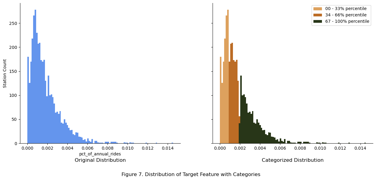
The main peak with a right skew was split into 3 equal categories based on percentileP. These categories were used to maintain constant distribution across the train and test sets.
Train Test Split (Remainder, Validation, Test)
For model training and hyperparameter tuning, the data were split into 4 sets:
1) test set: This data was reserved until all training and tuning was completed for final reporting.
2) remainder set: train + validation set, used for hyperparameter tuning after model is selected.
3) validation set: Used for selecting the most suitable model for hyperparameter tuning.
4) train set: Used for selecting the most suitable model for hyperparameter tuning.
# Reset index to make clean index after EDA
df.reset_index(inplace = True, drop = True)
The index of the data was reset for a clean row count after data cleaning. Then, the data was split with stratification using the 3 categories defined based on quantiles.
# Split data into remainder and test set
remainder_df, test_df = train_test_split(
    df,
    test_size = 0.1,
    stratify = df["pct_cat"],
    random_state = 42
)

# Further split remainder into validation and test
train_df, validation_df = train_test_split(
    remainder_df,
    test_size = 0.1,
    stratify = remainder_df["pct_cat"],
    random_state = 42
)
print(f"original data   : {df.shape[0]} rows and {df.shape[1]} columns.")
print(f"test data       : {test_df.shape[0]} rows and {test_df.shape[1]} columns.")
print(f"remainder data  : {remainder_df.shape[0]} rows and {remainder_df.shape[1]} columns.")
print(f"validation data : {validation_df.shape[0]} rows and {validation_df.shape[1]} columns.")
print(f"train data      : {train_df.shape[0]} rows and {train_df.shape[1]} columns.")
original data   : 3925 rows and 9 columns.
test data       : 393 rows and 9 columns.
remainder data  : 3532 rows and 9 columns.
validation data : 354 rows and 9 columns.
train data      : 3178 rows and 9 columns.
Now, a simple function was written to check if distribution is constant based on the categories:
# Define a simple function to check proportions by each category
def check_proportions(data, col):
    return np.round(data[col].value_counts() / len(data) *100,2)

compare_props = pd.DataFrame({
    "Original %"   : check_proportions(df,"pct_cat"),
    "Test %"       : check_proportions(test_df,"pct_cat"),
    "Remainder %"  : check_proportions(remainder_df,"pct_cat"),
    "Validation %" : check_proportions(validation_df,"pct_cat"),
    "Train %"      : check_proportions(train_df,"pct_cat")
    }
)

display(compare_props.head())
| Original % | Test % | Remainder % | Validation % | Train % | |
|---|---|---|---|---|---|
| pct_cat | |||||
| 67 - 100% quantile | 34.09 | 34.10 | 34.09 | 34.18 | 34.08 |
| 00 - 33% quantile | 33.07 | 33.08 | 33.07 | 33.05 | 33.07 |
| 34 - 66% quantile | 32.84 | 32.82 | 32.84 | 32.77 | 32.85 |
Based on the table above, it can be verified that the data has been split into various sets with the distribution of the target feature, pct_of_annual_rides preserved.
Model Selection
stn_lat and stn_lon, were the only 2 independent features available for prediction of the target variable pct_of_annual_rides. As latitude and longitude are descriptors of location, using them as continuous numerical features would be misrepresentative as a location with larger latitude is not necessarily larger or more important. Rather, the proximity of each station to cluster centers would be a better representation of the intuitive understanding of location. For example, a station being near a cluster center representing Mount Royal Park would be a better way to justify that station having more rides annually.
To this end, the KMeans clustering method was used to find cluster center for stations, with the similarity of each station to each cluster center measured using the Radial Basis Function(RBF).
- KMeans was chosen given the relatively small dataset and its simplicity of only 1 hyperparameter for tuning.
- RBF Kernel was chosen as the method for measuring the distance between each station and each cluster center because of its ability to determine how fast the similarity measure falls off using its hyperparameter, gamma.
Thus, KMeans and RBF Kernel were used to transform latitude and longitude into numerical features that can be fed into different models to predict pct_of_annual_rides. Although clustering metrics such as inertia and silhouette score can be used to measure how tight the clusters are, ultimately, the KMeans and RBF Kernel hyperparameters were tuned using Root Mean Square Error (RMSE) from the regression models.
Cluster Similarity Class
To begin, object oriented programming (OOP) was used to create a ClusterSimilarity class, which means that it will inherit the features of Scikit-Learn’s API, such as fit and fit_transform. Although not essential, this step makes building pipelines for hyperparameter tuning much neater.
# Create a class that combines KMeans with rbf_kernel to measure each station's similarity to the cluster center
class ClusterSimilarity(BaseEstimator, TransformerMixin):

    # Default number of KMeans clusters is 10, default RBF Kernel gamma is 1
    def __init__(self, n_clusters = 10, gamma = 1.0, random_state = None):
        self.n_clusters = n_clusters
        self.gamma = gamma
        self.random_state = random_state

    def fit(self, X, y = None, sample_weight = None):
        self.kmeans_ = KMeans(self.n_clusters, random_state = self.random_state, n_init = "auto")
        self.kmeans_.fit(X, sample_weight = sample_weight)
        return self

    def transform(self, X):
        return rbf_kernel(X, self.kmeans_.cluster_centers_, gamma = self.gamma)

    def get_feature_names_out(self, names = None):
        return [f"Cluster {i} similarity" for i in range(self.n_clusters)]
Below, the newly created ClusterSimilarity class was tested with 10 clusters. Note how the new class inherited the attributes of KMeans without explicit definition.
# Initiate a cluster similarity object
cluster_simil = ClusterSimilarity(
    n_clusters = 10,
    gamma = 1,
    random_state = 42
)

# Fit the cluster similarity object to the latitude and longitude columns
similarities = cluster_simil.fit_transform(remainder_df[["stn_lat","stn_lon"]])

# Initiate figure object
plt.figure()

# Plot the cluster centers by accessing the kmeans cluster center attribute
plt.plot(
    cluster_simil.kmeans_.cluster_centers_[:,0], # Latitude of cluster centre
    cluster_simil.kmeans_.cluster_centers_[:,1], # Longitude of cluster centre
    linestyle  = "",
    color      = "black",
    marker     = "X",
    markersize = 10,
    label      = "Cluster centers"
)

# Plot the latitude and longitude of stations in the remainder data
remainder_df.plot(
    kind  = "scatter",
    x     = "stn_lat",
    y     = "stn_lon",
    c     = "cornflowerblue",
    alpha = 0.2, # To deal with overlapping stations
    ax    = plt.gca()
)

# Tidy up plot
plt.legend()
plt.xlabel("Station Latitude")
plt.ylabel("Station Longitude")
sns.despine()
plt.title("Figure 8. Example of Cluster Centers Generated by KMeans", y = -0.2)
plt.show()
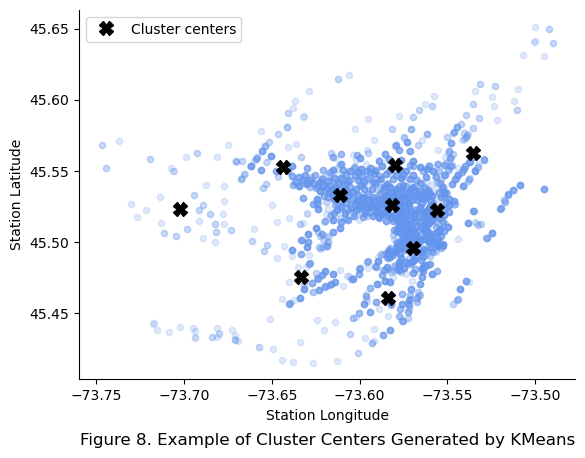
As expected, the new class also inherits the inertia attribute, which is a measure of the sum of squared distances from each point to the cluster centers as demonstrated below:
# Initiate empty lists to store values
k_val = []       # Number of cluster centers
inertia_val = [] # Inertia for each number of cluster centers

# Iterate through 15 values of cluster centers
for k in range(1,16):

    # Create ClusterSimilarity object with defined number of clusters
    cluster_simil = ClusterSimilarity(
        n_clusters = k,
        gamma = 1,
        random_state = 42
    )

    # Fit the Cluster Similarity object
    cluster_simil.fit_transform(remainder_df[["stn_lat","stn_lon"]])

    # Append attributes
    k_val.append(k)
    inertia_val.append(cluster_simil.kmeans_.inertia_)

# Visualize inertia values using scree plot
plt.figure()
plt.plot(k_val, inertia_val, marker="o")

# Define axis
plt.xlabel('Number of Clusters')
plt.ylabel('Inertia')
plt.title('Figure 9. Scree Plot for Various K-means Cluster Centers', y = -0.2)
sns.despine()

plt.show()
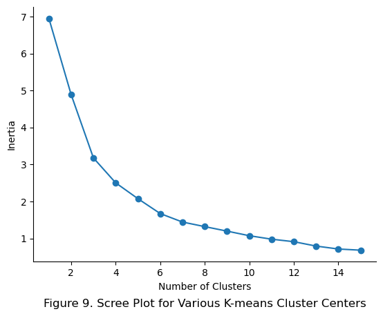
Although the scree plot shows that 10 clusters is relatively low on inertia compared to just 1 or 2 cluster centers, the final hyperparameter tuning will be done later using RMSE and GridSearchCV.
Preprocessing Column Transformer
Before selecting the model, the ClusterSimilarity class was combined with other preprocessing methods in a ColumnTransformer. A simple imputer using the median and a standard scaler were used to process numerical columns. As only two columns, each station’s latitude and longitude, were fed into the column transformer, the simple imputer and standard scaler were not used in this analysis, and were created for future analysis.
# Create ClusterSimilarity object
cluster_simil = ClusterSimilarity(
    n_clusters=10,
    gamma=1,
    random_state=42
)

# Create a pipeline that imputes any null values then feeds it through a standard scaler
num_pipeline = make_pipeline(
    SimpleImputer(strategy="median"),
    StandardScaler()
    )

# Combine numerical pipeline and ClusterSimilarity object into a column transformer.
preprocessing = ColumnTransformer(
    [
        ("stn_loc", cluster_simil, ["stn_lat","stn_lon"])
    ],
    remainder = num_pipeline
)
The transformer was tested using the remainder data.
# Test the column transformer pipeline
remainder_prepared = preprocessing.fit_transform(remainder_df[["stn_lat", "stn_lon"]])

# Examine data before column transformer
print(f"Before preprocessing pipeline")
display(remainder_df[["stn_lat", "stn_lon"]].head())

# Examine data after column transformer
print(f"After preprocessing pipeline")

# Extract column names from preprocessing pipeline
processed_remainder_df = pd.DataFrame(
    remainder_prepared,
    columns = preprocessing.get_feature_names_out(),
    index = remainder_df.index
)

display(processed_remainder_df.head())
Before preprocessing pipeline
| stn_lat | stn_lon | |
|---|---|---|
| 1424 | 45.493909 | -73.559507 |
| 2567 | 45.471926 | -73.582470 |
| 2512 | 45.550698 | -73.609530 |
| 1842 | 45.520604 | -73.575984 |
| 2356 | 45.472503 | -73.539285 |
After preprocessing pipeline
| stn_loc__Cluster 0 similarity | stn_loc__Cluster 1 similarity | stn_loc__Cluster 2 similarity | stn_loc__Cluster 3 similarity | stn_loc__Cluster 4 similarity | stn_loc__Cluster 5 similarity | stn_loc__Cluster 6 similarity | stn_loc__Cluster 7 similarity | stn_loc__Cluster 8 similarity | stn_loc__Cluster 9 similarity | |
|---|---|---|---|---|---|---|---|---|---|---|
| 1424 | 0.999153 | 0.995976 | 0.989462 | 0.994232 | 0.995808 | 0.999893 | 0.994748 | 0.998497 | 0.979020 | 0.998324 |
| 2567 | 0.996720 | 0.993267 | 0.989735 | 0.997415 | 0.995443 | 0.999260 | 0.989657 | 0.997097 | 0.983171 | 0.999878 |
| 2512 | 0.996372 | 0.999105 | 0.998815 | 0.993763 | 0.999690 | 0.995419 | 0.994366 | 0.998599 | 0.990748 | 0.991329 |
| 1842 | 0.999599 | 0.998866 | 0.994365 | 0.994678 | 0.998611 | 0.999351 | 0.996609 | 0.999942 | 0.984222 | 0.996389 |
| 2356 | 0.997191 | 0.991739 | 0.982754 | 0.991204 | 0.991204 | 0.998531 | 0.991952 | 0.995382 | 0.971312 | 0.997882 |
The preprocessing pipeline worked as expected. The latitude and longitude columns were converted to similarity measures of each station to each of the 10 cluster centers discovered from the KMeans clustering method.
Model Pipeline
The preprocessing ColumnTransformer was then included as part of a modelling pipeline. Before testing models with no hyperparameter tuning, a function was written to reduce repetitive code.
def base_model_fit(X_tr, y_tr, X_va, y_va, model_object):
    '''
    Fits a model using default parameters and returns remainder and test root mean square errors(RMSE).
    Remainder: train + validation data

    Usecase in project: used to build the base model of each classifier

    Input
    -----
    X_tr : train independent variables
    y_tr : train dependent variables
    X_va : validation set independent variables
    y_va : validation set dependent variables
    model_object : sklearn models such as DecisionTreeClassifier()

    Output
    ------
    Remainder RMSE
    Test RMSE
    Time taken (seconds)
    '''
    # Start timer
    start = time.perf_counter()

    # Initiate the model with no parameters set
    # Note preprocessing defaults to 10 KMeans cluster centers and a RBF Kernel gamma of 1
    model = make_pipeline(preprocessing, model_object)

    # Fit the model
    model.fit(X_tr,y_tr)

    # Evaluate the prediction
    y_tr_pred = model.predict(X_tr)
    y_va_pred = model.predict(X_va)

    # Evaluate the RMSE
    model_tr_rmse = mean_squared_error(y_tr,y_tr_pred, squared = False)
    model_va_rmse = mean_squared_error(y_va, y_va_pred, squared = False)

    # Print the train and validation scores
    print(f"Base fitting of a {str(model)} with no hyperparameter adjustment.")
    print(f"RMSE for train data: {np.round(model_tr_rmse*100,3)}%")
    print(f"RMSE for validation data: {np.round(model_va_rmse*100,3)}%")

    # End timmer
    end = time.perf_counter()
    time_taken = np.round(end-start,4)
    print(f"Time taken:{time_taken} seconds")
    return model
Then, the split data from the stratification processed was renamed for neatness.
# Split the train and validation sets into more conventional X and y labelling
X_tr = train_df[["stn_lat","stn_lon"]]
y_tr = train_df["pct_of_annual_rides"]

# Validation set
X_va = validation_df[["stn_lat","stn_lon"]]
y_va = validation_df["pct_of_annual_rides"]
Model Testing
Linear Regression
To start, the simple Linear Regression model was used.
# Fit basic LinearRegression model
model_01 = base_model_fit(X_tr, y_tr, X_va, y_va, LinearRegression())
Base fitting of a Pipeline(steps=[('columntransformer',
                 ColumnTransformer(remainder=Pipeline(steps=[('simpleimputer',
                                                              SimpleImputer(strategy='median')),
                                                             ('standardscaler',
                                                              StandardScaler())]),
                                   transformers=[('stn_loc',
                                                  ClusterSimilarity(gamma=1,
                                                                    random_state=42),
                                                  ['stn_lat', 'stn_lon'])])),
                ('linearregression', LinearRegression())]) with no hyperparameter adjustment.
RMSE for train data: 0.125%
RMSE for validation data: 0.128%
Time taken:0.3154 seconds
To give context, most stations range between 0.073% to 0.243% of annual rides, so a validation error of 0.128% does not provide much confidence for the base LinearRegression() model.
# Context for understanding mean square error
df["pct_of_annual_rides"].describe()*100
count    392500.000000
mean          0.178344
std           0.150042
min           0.000018
25%           0.073391
50%           0.138250
75%           0.243030
max           1.453954
Name: pct_of_annual_rides, dtype: float64
Decision Tree Regressor
# Fit basic Decision Tree Regressor
model_02 = base_model_fit(X_tr,y_tr,X_va,y_va, DecisionTreeRegressor(random_state = 42))
Base fitting of a Pipeline(steps=[('columntransformer',
                 ColumnTransformer(remainder=Pipeline(steps=[('simpleimputer',
                                                              SimpleImputer(strategy='median')),
                                                             ('standardscaler',
                                                              StandardScaler())]),
                                   transformers=[('stn_loc',
                                                  ClusterSimilarity(gamma=1,
                                                                    random_state=42),
                                                  ['stn_lat', 'stn_lon'])])),
                ('decisiontreeregressor',
                 DecisionTreeRegressor(random_state=42))]) with no hyperparameter adjustment.
RMSE for train data: 0.038%
RMSE for validation data: 0.065%
Time taken:0.3023 seconds
As expected for a decision tree with unlimited depth, the model has overfitted over the train data, explaining why the RMSE for validation data was almost double of the RMSE for train data. The performance in time was similar to LinearRegression.
Random Forest Regressor
model_03 = base_model_fit(X_tr, y_tr, X_va, y_va, RandomForestRegressor(random_state = 42))
Base fitting of a Pipeline(steps=[('columntransformer',
                 ColumnTransformer(remainder=Pipeline(steps=[('simpleimputer',
                                                              SimpleImputer(strategy='median')),
                                                             ('standardscaler',
                                                              StandardScaler())]),
                                   transformers=[('stn_loc',
                                                  ClusterSimilarity(gamma=1,
                                                                    random_state=42),
                                                  ['stn_lat', 'stn_lon'])])),
                ('randomforestregressor',
                 RandomForestRegressor(random_state=42))]) with no hyperparameter adjustment.
RMSE for train data: 0.041%
RMSE for validation data: 0.066%
Time taken:2.3212 seconds
As expected of an ensemble model, the ensemble of decision trees produces a model that is less overfit on the train data compared to just a single decision tree. The time taken was observed to be roughly 7 times the time taken by a decision tree model.
Support Vector Regressor
model_04 = base_model_fit(X_tr, y_tr, X_va, y_va, SVR())
Base fitting of a Pipeline(steps=[('columntransformer',
                 ColumnTransformer(remainder=Pipeline(steps=[('simpleimputer',
                                                              SimpleImputer(strategy='median')),
                                                             ('standardscaler',
                                                              StandardScaler())]),
                                   transformers=[('stn_loc',
                                                  ClusterSimilarity(gamma=1,
                                                                    random_state=42),
                                                  ['stn_lat', 'stn_lon'])])),
                ('svr', SVR())]) with no hyperparameter adjustment.
RMSE for train data: 0.569%
RMSE for validation data: 0.57%
Time taken:0.2038 seconds
Given the relatively small dataset (<5,000 rows), a support vector machine model was tested to produce a model that was well fitted to both train and validation data at the fastest time.
Summary of Model Selection
| Model | Model_type | RMSE_train | RMSE_validation | Time |
|---|---|---|---|---|
| model_01 | LinearRegression() | 0.125% | 0.128% | 0.3154 |
| model_02 | DecisionTreeRegressor() | 0.038% | 0.065% | 0.3023 |
| model_03 | RandomForestRegressor() | 0.041% | 0.066% | 2.3212 |
| model_04 | SVR() | 0.569% | 0.570% | 0.2038 |
Based on the summarized results of quickly testing multiple models, the random forest regressor was chosen to proceed with hyperparameter tuning. The decision tree and random forest regressors performed better compared to other models in terms of validation RMSE. The observed gap between train and validation RMSE for both tree regressors were expected due to decision trees overfitting when max depth is not controlled. This can be reduced using cross validation during hyperparameter optimization. With the assumption that station usage planning happens only a few times a year, the higher time consumed by the random forest regressor was deemed acceptable given that an ensemble of decision trees will be more generalizable to the data compared to just a single decision tree.
Hyperparameter Tuning
The goals of hyperparameter tuning are to find the model hyperparameters that provide an optimum balance between model fit to available data and its ability to generalize to new data. The following hyperparameters will be tuned through the use of grid search and cross validation (GridSearchCV):
1) n_clusters: Number of clusters from KMeans clustering of station locations
2) gamma: The rate at which similarity falls off when comparing each station to cluster centers from KMeans
3) max_features: This hyperparameter limits the number of randomly selected features each node considers for splitting in each decision tree within the random forest.
# Extract the independent and dependent variables into X and y for readability
X_re = remainder_df[["stn_lat", "stn_lon"]]
y_re = remainder_df["pct_of_annual_rides"]
Round 1
To start, a grid of 5 values for each hyperparameter was tested. Given a cross validation of 3 folds, the total number of model fittings performed will be 375 fits. Given the relative small data size (<5,000 rows) and only 3 hyperparameters to optimize, GridSearchCV was used over RandomizedSearchCV for its simplicity.
# Build pipeline which GridSearchCV will run for each fit
pipeline = Pipeline(
    [
        ("preprocessing", preprocessing),
        ("random_forest", RandomForestRegressor(random_state = 42))
    ]
)

# Generate a grid of parameters for which gridsearchCV will test all combinations of parameters
param_grid = [
    {
        "preprocessing__stn_loc__n_clusters": [5, 10, 15, 20, 25],
        "preprocessing__stn_loc__gamma": [0.01, 0.1, 1, 10, 100],
        "random_forest__max_features": [3, 5, 7, 9, 12]
    }
]

# Build the grid search object
grid_search = GridSearchCV(
    pipeline,
    param_grid = param_grid,
    verbose = 5,
    n_jobs = -1,   # Use all processors available
    refit = False, # False = to not refit model with best parameters on the whole dataset
    cv = 3,        # 3 fold cross-validation
    scoring = "neg_root_mean_squared_error"
)

# Perform the grid search on remainder dataset
with print_time():
    grid_search.fit(X_re, y_re)
Fitting 3 folds for each of 125 candidates, totalling 375 fits
Time taken: 67.0657 seconds.
The grid search and cross validation process for 375 fits took only 65 seconds in this study, which is acceptable considering this process is most likely an annual process. The best parameters can be extracted from the grid search by accessing the best_params_ attribute.
# Examine the best hyperparameters
grid_search.best_params_
{'preprocessing__stn_loc__gamma': 100,
 'preprocessing__stn_loc__n_clusters': 25,
 'random_forest__max_features': 9}
The best gamma and n_clusters hyperparameter were found to be on the right end of provided values, warranting a further grid search for values that are beyond the right boundaries. The best max_features hyperparameter was 9. This hyperparameter only has effect when the the number of KMeans clusters is greater than 9, meaning that the best n_clusters of 25 makes sense. Before moving on to the next round, the RMSE errors were examined in greater detail through the cv_results attribute.
# Store the gridsearch results into a DataFrame
cv_res = pd.DataFrame(grid_search.cv_results_)

# Sort by mean test score in descending order since the values are negative RMSE
cv_res.sort_values(
    by = "mean_test_score", ascending = False, inplace = True
)

# Select specific columns for review
cv_res = cv_res.loc[:,[
    "param_preprocessing__stn_loc__gamma",
    "param_preprocessing__stn_loc__n_clusters",
    "param_random_forest__max_features",
    "split0_test_score",
    "split1_test_score",
    "split2_test_score",
    "mean_test_score"
]]

# Specify column names for renaming
score_cols = ["split0","split1","split2","mean_test_rmse"]

# Rename the columns in DataFrame for readability
cv_res.columns = ["gamma", "n_clusters", "max_features"] + score_cols

# For the score columns, multiply by negative to get positive RMSE, then multiply by 100 to convert to percentages
cv_res[score_cols] = -cv_res[score_cols]*100

# Examine the first 10 results
print(f"Hyperparameter Optimization Round 1: The Top 10 Hyperparameter Combinations based on Ascending RMSE:")
cv_res.head(10)
Hyperparameter Optimization Round 1: The Top 10 Hyperparameter Combinations based on Ascending RMSE:
| gamma | n_clusters | max_features | split0 | split1 | split2 | mean_test_rmse | |
|---|---|---|---|---|---|---|---|
| 123 | 100 | 25 | 9 | 0.062646 | 0.070340 | 0.070507 | 0.067831 |
| 122 | 100 | 25 | 7 | 0.062616 | 0.070230 | 0.070735 | 0.067860 |
| 46 | 0.1 | 25 | 5 | 0.062804 | 0.070334 | 0.070656 | 0.067931 |
| 96 | 10 | 25 | 5 | 0.062669 | 0.070139 | 0.071097 | 0.067969 |
| 74 | 1 | 25 | 12 | 0.062594 | 0.070449 | 0.071089 | 0.068044 |
| 97 | 10 | 25 | 7 | 0.062821 | 0.070062 | 0.071258 | 0.068047 |
| 110 | 100 | 15 | 3 | 0.062723 | 0.070378 | 0.071073 | 0.068058 |
| 45 | 0.1 | 25 | 3 | 0.062775 | 0.070357 | 0.071054 | 0.068062 |
| 104 | 100 | 5 | 12 | 0.064152 | 0.069341 | 0.070739 | 0.068077 |
| 103 | 100 | 5 | 9 | 0.064152 | 0.069341 | 0.070739 | 0.068077 |
7 of the top 10 hyperparameter had 25 as the number of clusters, further warranting a second grid search to explore the hyperparameter values to the right of the boundaries in the first grid search. It was worth noting that the best mean RMSE score was worse than the base model with no hyperparameter tuning (model_03, validation RMSE 0.066%). However, this lower RMSE was prefered as it produces a model that is more generizable to new data, not just to the data it was trained upon.
Round 2
In round 2, aside from increasing the hyperparameter values to the right of their boundaries in round 1, a smaller step size will also be used in the hopes of finding an optimal combination that is within the middle of the hyperparameter values to be tested in round 2.
# Build pipeline which GridSearchCV will run
pipeline = Pipeline(
    [
        ("preprocessing", preprocessing),
        ("random_forest", RandomForestRegressor(random_state = 42))
    ]
)

# Generate a grid of parameters for which gridsearchCV will test all combinations of parameters
param_grid = [
    {
        "preprocessing__stn_loc__n_clusters": np.arange(23, 28, 1),
        "preprocessing__stn_loc__gamma": np.arange(500,2600,500),
        "random_forest__max_features": np.arange(7, 12, 1)
    }
]

# Build the grid search object
grid_search = GridSearchCV(
    pipeline,
    param_grid = param_grid,
    verbose = 5,
    n_jobs = -1,   # Use all processors available
    refit = False, # False = to not refit model with best parameters on the whole dataset
    cv = 3,        # 3 fold cross-validation
    scoring = "neg_root_mean_squared_error"
)

# Perform the grid search on remainder dataset
with print_time():
    grid_search.fit(X_re, y_re)
Fitting 3 folds for each of 125 candidates, totalling 375 fits
Time taken: 73.7823 seconds.
# Examine the best params
grid_search.best_params_
{'preprocessing__stn_loc__gamma': 1000,
 'preprocessing__stn_loc__n_clusters': 25,
 'random_forest__max_features': 8}
The best hyperparameters from round 2 were in the middle of each hyperparameter’s list of value to be tested, suggesting that an optimal hyperparameter combination had been found. Before finalizing the hyperparameters, the grid search results were again reviewed through a DataFrame.
# Store the gridsearch results into a DataFrame
cv_res = pd.DataFrame(grid_search.cv_results_)

# Sort by mean test score in descending order since the values are negative RMSE
cv_res.sort_values(
    by = "mean_test_score", ascending = False, inplace = True
)

# Select specific columns for review
cv_res = cv_res.loc[:,[
    "param_preprocessing__stn_loc__gamma",
    "param_preprocessing__stn_loc__n_clusters",
    "param_random_forest__max_features",
    "split0_test_score",
    "split1_test_score",
    "split2_test_score",
    "mean_test_score"
]]

# Specify column names for renaming
score_cols = ["split0","split1","split2","mean_test_rmse"]

# Rename the columns in DataFrame for readability
cv_res.columns = ["gamma", "n_clusters", "max_features"] + score_cols

# For the score columns, multiply by negative to get positive RMSE, then multiply by 100 to convert to percentages
cv_res[score_cols] = -cv_res[score_cols]*100

# Examine the first 10 results
print(f"Hyperparameter Optimization Round 1: The Top 10 Hyperparameter Combinations based on Ascending RMSE:")
cv_res.head(10)
Hyperparameter Optimization Round 1: The Top 10 Hyperparameter Combinations based on Ascending RMSE:
| gamma | n_clusters | max_features | split0 | split1 | split2 | mean_test_rmse | |
|---|---|---|---|---|---|---|---|
| 36 | 1000 | 25 | 8 | 0.062236 | 0.069939 | 0.070925 | 0.067700 |
| 23 | 500 | 27 | 10 | 0.062789 | 0.069672 | 0.070651 | 0.067704 |
| 22 | 500 | 27 | 9 | 0.062817 | 0.069792 | 0.070555 | 0.067722 |
| 9 | 500 | 24 | 11 | 0.062724 | 0.069469 | 0.071291 | 0.067828 |
| 86 | 2000 | 25 | 8 | 0.062548 | 0.070026 | 0.070922 | 0.067832 |
| 59 | 1500 | 24 | 11 | 0.062470 | 0.069974 | 0.071100 | 0.067848 |
| 53 | 1500 | 23 | 10 | 0.062411 | 0.070110 | 0.071091 | 0.067871 |
| 71 | 1500 | 27 | 8 | 0.062370 | 0.070898 | 0.070350 | 0.067873 |
| 11 | 500 | 25 | 8 | 0.062870 | 0.070030 | 0.070732 | 0.067877 |
| 74 | 1500 | 27 | 11 | 0.062417 | 0.070399 | 0.070835 | 0.067884 |
| Round | Best gamma |
Best n_clusters |
Best max_features |
Mean RMSE |
|---|---|---|---|---|
| No tuning | 1 | 10 | 10 | 0.066% (Validation) |
| 1 | 100 | 25 | 9 | 0.0678% |
| 2 | 1000 | 25 | 8 | 0.0677% |
In round 2 of hyperparameter optimization, the higher gamma suggests a quicker falloff in similarity when comparing each station’s locations to the cluster centers. Given that most Bixi stations are within the island of Montreal, the high gamma allows the model to better differentiate stations that are relatively close to each other. However, the high gamma value may also mean that a station which is far away from all 25 cluster centers would receive a low similarity score across all stations. This potential problem will be explored later when visually analyzing the cluster centers.
The max_features of 8 suggests that the best model looks at only a max of 8 cluster centers when making a split at each node. Surprisingly, this is similar to human intuition of recognizing city locations based on its proximity to just a few landmarks, rather than referring to all the landmarks in the city before recognizing a location.
Further hyperparameter tuning can be perfomed to find an even more optimized combination of hyperparameters. However, given that 2 rounds of tuning showed negligible improvement in RMSE, the 2 rounds were deemed sufficient to prepare a model that is generizable to new data, and, is not overfitted on the remainder data.
Evaluation of Final Model
The best hyperparameters were used to build a final model in a simlar fashion to hyperparameter tuning, except only 1 combination of hyperparameters were provided and refit was set to True. Further analysis was performed on the final model before moving on to test it with the reserved test data for reporting.
# Insert best parameters into a parameter grid
final_param_grid = param_grid = [
    {
        "preprocessing__stn_loc__n_clusters": [25],
        "preprocessing__stn_loc__gamma": [1000],
        "random_forest__max_features": [8]
    }
]

# Use grid search to fit the model with the final parameters
grid_search = GridSearchCV(
    pipeline,
    param_grid = final_param_grid,
    verbose = 5,
    n_jobs = -1,
    refit = True,
    cv = 3,
    scoring = "neg_root_mean_squared_error"
)

# Perform the fit
grid_search.fit(X_re, y_re)

# Store the best estimator as the final model
final_model = grid_search.best_estimator_
Fitting 3 folds for each of 1 candidates, totalling 3 fits
Cluster Centers
The 25 cluster centers were accessed through the transformers_ attribute of the final model.
# cc_df: cluster center DataFrame
cc_df = pd.DataFrame({
    "cluster_name" : final_model["preprocessing"].get_feature_names_out(),
    "cluster_lat"  : final_model["preprocessing"].transformers_[0][1].kmeans_.cluster_centers_[:,0],
    "cluster_lon"  : final_model["preprocessing"].transformers_[0][1].kmeans_.cluster_centers_[:,1]
})

# # For simplicity, the cluster names are reduced to just the number within each string
# cc_df["cluster_name"] = cc_df["cluster_name"].str.extract('(\d+)').astype("int")+1

display(cc_df.head())
| cluster_name | cluster_lat | cluster_lon | |
|---|---|---|---|
| 0 | stn_loc__Cluster 0 similarity | 45.506621 | -73.573372 |
| 1 | stn_loc__Cluster 1 similarity | 45.552163 | -73.575543 |
| 2 | stn_loc__Cluster 2 similarity | 45.559606 | -73.652577 |
| 3 | stn_loc__Cluster 3 similarity | 45.445015 | -73.596257 |
| 4 | stn_loc__Cluster 4 similarity | 45.540311 | -73.623883 |
Furthermore, the relative importance of each cluster center can be extracted from the final model using the feature_importances attribute. This measure of importance is calculated by examining how much the tree nodes which used that feature reduce impurity on average across all 100 decision trees in the final model. This measure of importance is scaled such that the sum across all features adds up to 1.
For ease of reference each cluster center, the cluster centers were renamed based on their importance.
# Get importance of each cluster center from final model
cc_df["importance"] = final_model["random_forest"].feature_importances_

# order by feature importance
cc_df.sort_values(
    by = ["importance"],
    ascending = [False],
    inplace =  True
)

# Number of clusters (ascending)
cc_df["cluster_name"] = cc_df["importance"].rank(ascending = False).astype("int")

# Cumulative importance
cc_df["cum_importance"] = cc_df["importance"].cumsum()

# Reset index for neatness
cc_df.reset_index(drop = True, inplace = True)

# Examine the top 10 cluster centers
display(cc_df.head(10))
| cluster_name | cluster_lat | cluster_lon | importance | cum_importance | |
|---|---|---|---|---|---|
| 0 | 1 | 45.506621 | -73.573372 | 0.130542 | 0.130542 |
| 1 | 2 | 45.510082 | -73.558289 | 0.096973 | 0.227515 |
| 2 | 3 | 45.529592 | -73.576008 | 0.069114 | 0.296629 |
| 3 | 4 | 45.489861 | -73.568448 | 0.065767 | 0.362396 |
| 4 | 5 | 45.499491 | -73.630374 | 0.064089 | 0.426484 |
| 5 | 6 | 45.445015 | -73.596257 | 0.057919 | 0.484403 |
| 6 | 7 | 45.516432 | -73.691777 | 0.054201 | 0.538604 |
| 7 | 8 | 45.457505 | -73.574330 | 0.046285 | 0.584889 |
| 8 | 9 | 45.513747 | -73.529658 | 0.040833 | 0.625722 |
| 9 | 10 | 45.523794 | -73.611104 | 0.036474 | 0.662196 |
The cluster centers were plotted along with the cumulative importance.
# Initiate figure object
plt.figure()

# Create line plot
cc_df.plot(
    x = "cluster_name",
    y = "cum_importance",
    kind = "line",
    ax = plt.gca(),
    legend = False
)

# Define location for annotation
ann_x = 15
ann_y = cc_df.loc[cc_df["cluster_name"] == 15,"cum_importance"].values[0]

# Plot a marker to highlight 80% cumulated importance
plt.plot(
    ann_x,
    ann_y,
    marker = ".",
    markersize = 10,
    color = "black"
)

# Add annotations
plt.annotate(
    text = "80% of cumulated importance \nexplained by 15 cluster centers",
    xy = (ann_x,ann_y),
    xytext = (ann_x*1.05, ann_y*0.70),
    arrowprops = dict(facecolor = "black", shrink = 0.05)
)

# Tidy up plot
plt.ylabel(f"Cumulative Sum of Feature Importance")
plt.xlabel(f"Number of Clusters, sorted by desc Feature Importance")
plt.title(f"Figure 10. Cumulative Importance vs Number of Clusters", y = -0.2)
sns.despine()
plt.show()
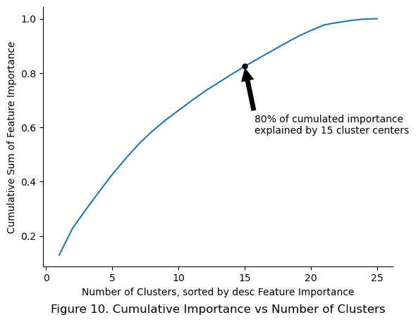
80% of cumulative importance was explained by the top 15 cluster centers. Further experiments maybe conducted to determine how much performance drops if only 15 cluster centers were used instead.
Then, the cluster centers were plotted against the station locations for a geo-visual understanding of the cluster centers. The size of markers represent the importance of the cluster center in the final models perspective.
# Initiate figure object
plt.figure()

# Plot the latitude and longitude of stations in the remainder data
remainder_df.plot(
    kind  = "scatter",
    y     = "stn_lat",
    x     = "stn_lon",
    c     = "cornflowerblue",
    alpha = 0.2, # To deal with overlapping stations
    ax    = plt.gca()
)

# Plot the cluster centers
cc_df.plot(
    kind = "scatter",
    y = "cluster_lat",
    x = "cluster_lon",
    color = "black",
    linestyle = "",
    marker = "X",
    label = "Cluster centers",
    s = cc_df["importance"]*1000,
    ax = plt.gca())

# Annotate each cluster center
annotations = [plt.annotate(label, (cc_df["cluster_lon"][i], cc_df["cluster_lat"][i])) for i, label in enumerate(cc_df["cluster_name"])]

# Tidy annotation position
adjust_text(annotations)

# Tidy plot
sns.despine()
plt.xlabel(f"Station Longitude")
plt.ylabel(f"Station Latitude")
plt.title("Figure 11. Cluster Centers Generated by Final Model", y = -0.2)
plt.show()
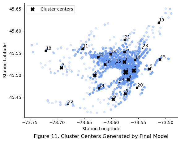
The top 10 cluster centers in terms of importance were observed to be roughly evenly spread out across the city rather than being clumped together in the city center of Montreal. Many cluster centers that are not in the top 10 were also found around to be in the city center of Montreal. This suggests that the final model is dependent on these less important feature to finely differentiate stations in between the top 10 stations.
A deeper interactive visualization using plotly was also used to explore the cluster centers identified by the model.
# Read in mapbox secret from .mapbox_token file
px.set_mapbox_access_token(open("../.mapbox_token").read())

# Create plotly express map object for the station lat and lon
fig = px.scatter_mapbox(
    remainder_df,
    lat        = "stn_lat",
    lon        = "stn_lon",
    text       = "stn_name",
    title      = "Figure 12. Cluster Centers from Final Model Overlayed over Montreal",
    hover_name = "stn_name",
    hover_data = {
        "rides" : ":,",
        "stn_lat" : ":.3f",
        "stn_lon" : ":.3f",
    },
    zoom       = 10.7,
    opacity    = 0.1
)

# Add plotly trace for cluster centers from final model
fig.add_scattermapbox(
    lat      = cc_df["cluster_lat"],
    lon      = cc_df["cluster_lon"],
    text     = [str(name) for name in cc_df["cluster_name"]],
    mode     = "text",
    textfont = {"size":25}
)

# Tidy up layout of figure
fig.update_layout(
    # Set title
    title = dict(
        x = 0.5,
        y = 0.05
    ),
    autosize   = False,
    width      = 1000,
    height     = 1000,
    showlegend = False
)

fig.show()
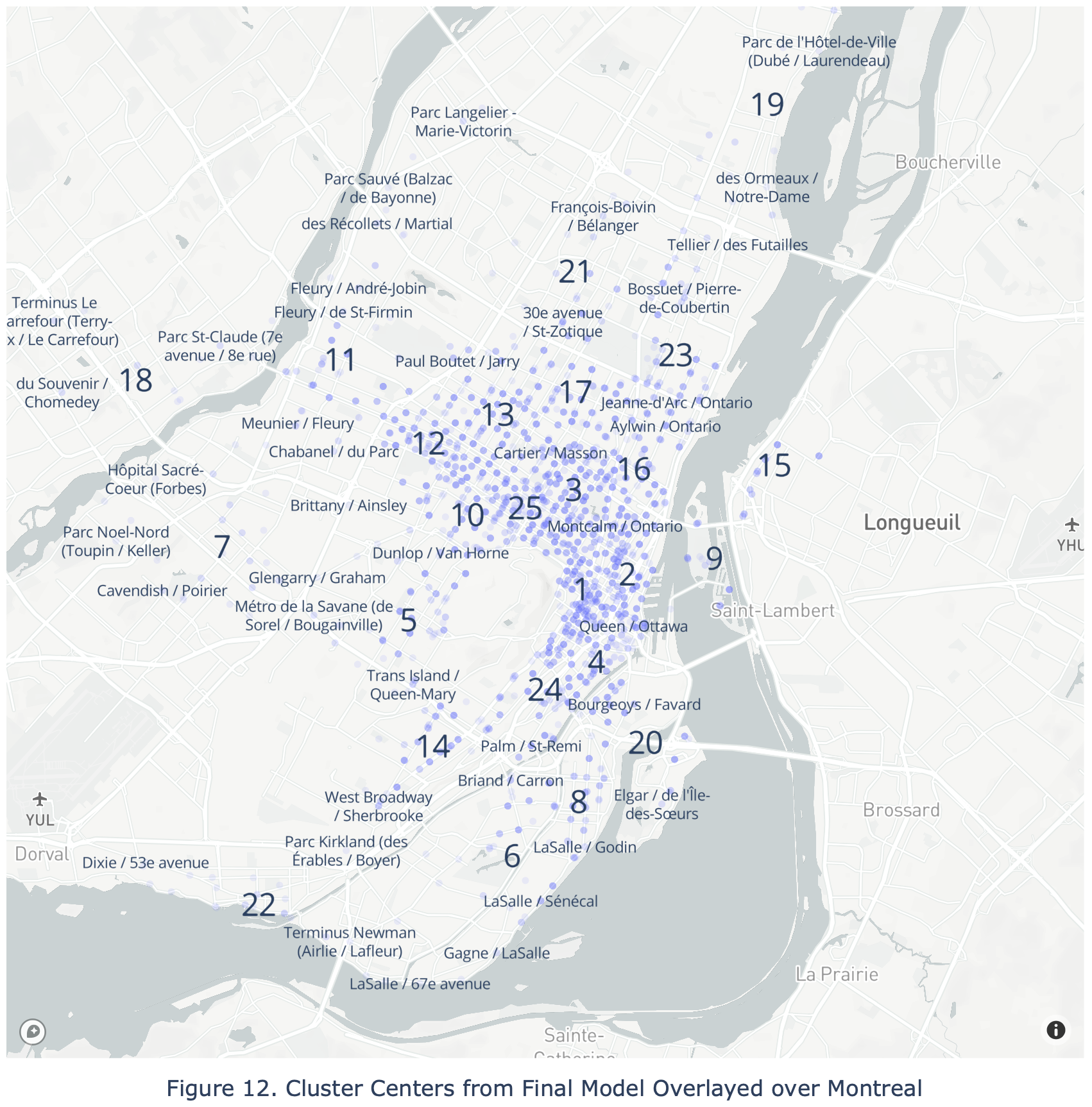
Overlaying the cluster centers over an actual map of Montreal reveals that the most important cluster is centered around McGill University, likely due to the large amounts of bicycle traffic by students. Further detailed analysis for each cluster center with its surrounding landmarks was now possible, but not included in this article for brevity.
Final Evaluation
For final reporting, the trained model was evaluated using the test set, which had been excluded throughout the entire model training process.
# Extract the independent and dependent variables into X and y for readability
X_te = test_df[["stn_lat", "stn_lon"]]
y_te = test_df["pct_of_annual_rides"]

# Generate final predictions
final_predictions = final_model.predict(X_te)

# Calculate and display final RMSE error
final_rmse = mean_squared_error(y_te, final_predictions, squared = False)
print(f"Final RMSE: {np.round(final_rmse * 100,5)} %")
Final RMSE: 0.05608 %
To better represent the confidence in a model’s prediction, the 95% confidence interval calculated below.
# Define confidence interval
confidence = 0.95

# Define squared errors
squared_errors = (final_predictions - y_te) **2

# Calculate a 95 % confidence interval
ci = np.sqrt(
    stats.t.interval(
        confidence,
        len(squared_errors) - 1,
        loc = squared_errors.mean(),
        scale = stats.sem(squared_errors)
    )
)*100

print(f"Final RMSE: {np.round(final_rmse * 100,5)} % with a 95% CI of {np.round(ci,5)} %.")
Final RMSE: 0.05608 % with a 95% CI of [0.0477 0.06336] %.
The final model was able to predict the percentage of annual rides for each station given its latitude and longitude with a RMSE of 0.05608%. To better understand what this implies, the final error was analyzed against the 3 categories created in the stratification step.
# Display range of "percentage of annual rides" for each station
print(f"The distribution of `percentage of annual rides` in % by Percentiles")
df.groupby(by = "pct_cat")["pct_of_annual_rides"].describe().iloc[:,3:].T*100
The distribution of `percentage of annual rides` in % by Percentiles
| pct_cat | 00 - 33% percentile | 34 - 66% percentile | 67 - 100% percentile |
|---|---|---|---|
| min | 0.000018 | 0.091008 | 0.197032 |
| 25% | 0.031090 | 0.112905 | 0.239177 |
| 50% | 0.055255 | 0.136307 | 0.301887 |
| 75% | 0.073105 | 0.162927 | 0.393963 |
| max | 0.091000 | 0.196958 | 1.453954 |
For the first category, the 00-33% percentile, the final model’s RMSE was larger than the median (0.05608% > 0.055255%), which means the model will likely perform poorly for stations with little to no annual usage.
As the second and third categories represent stations with greater usage, the final model’s RMSE suggests it performs best when predicting the percentage of annual rides for stations with the higest number of rental trips.
Finally, to evaluate the model’s ability to predict the number of Bixi trips across the years based on station location, the final model used to predict the percentage of annual rides for each station, which was then multiplied by the total rides for each year. The result was then summed and compared to the actual number of rides each year in a bar chart.
# Store station location and latitudes into a neat variable X
X = df[["stn_lat","stn_lon"]]

# Generate predictions using the final model
with print_time():
    y_pr = final_model.predict(X)
Time taken: 0.1011 seconds.
# Store the final predictions in DataFrame
df["pred_pct_of_annual_rides"] = y_pr
df["pred_rides"] = df["pred_pct_of_annual_rides"] * df.groupby(by = ["year"])["rides"].transform("sum")
# Create a pivot table summarizing the actual number of trips per year and predicted number of trips
plot_df = df.groupby(
    by = ["year"],
    as_index = False
).agg(
    actual_trips = ("rides","sum"),
    predicted_trips = ("pred_rides","sum")
)

# Define x-axis, bar width, and multiplier for counting bar position
x = plot_df["year"].unique()
width = 0.25
multiplier = 0

# Create a plot summarizing the actual number of trips per year and predicted number of trips
fig, ax = plt.subplots(
    layout = "constrained"
)

for attribute, measurement in plot_df[["actual_trips", "predicted_trips"]].items():
    offset = width * multiplier
    rects = ax.bar(x + offset, np.round(measurement/1_000_000,1), width, label=attribute)
    ax.bar_label(rects, padding=4, rotation = 90)
    multiplier += 1

# Tidy up the plot
ax.set_xlabel(f"Year")
ax.set_ylabel(f"Number of Trips (millions)")
ax.set_title(f"Figure 13. Predicted Rides for each Year", y = -0.2)
ax.legend(loc='upper left', ncols=3)

sns.despine()
plt.show()
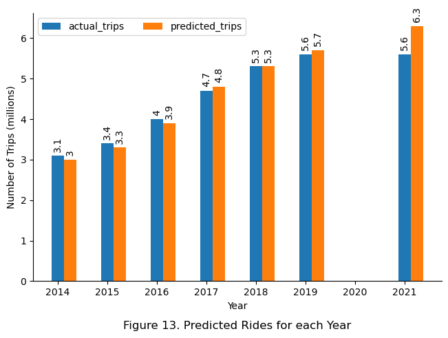
Although the final model was observed to perform unsatisfactorily for stations with number of trips in the 0-33% quantile, the overall performance of the final model on an annual basis suggests otherwise. The model was able to predict the number of trips accurately within 0.1 million trips for the years 2014 to 2019, only deviating significantly by 0.7 million trips for the year 2021. This is likely due to the errors for stations with little trips being insignificant compared to more busy stations, thus offering little to no effect on the overall annual sum. The deviation in 2021 might be due to the effects of recovery from Covid-19, but further detailed analysis was required to verify this. In retrospect, the difference observed in 2021 might suggest that the model has not learned the one-time effect of the Covid-19 pandemic, which would make it more generizable to new data.
# Final numerical check that the final model was actually making predictions
display(df.loc[0:5, ["year", "start_stn_code", "rides","pred_rides"]].round(0))
| year | start_stn_code | rides | pred_rides | |
|---|---|---|---|---|
| 0 | 2021 | 10 | 4478.0 | 3855.0 |
| 1 | 2021 | 100 | 6871.0 | 5768.0 |
| 2 | 2021 | 1000 | 1093.0 | 1140.0 |
| 3 | 2021 | 1002 | 4469.0 | 5642.0 |
| 4 | 2021 | 1003 | 3179.0 | 3134.0 |
| 5 | 2021 | 1004 | 1383.0 | 1035.0 |
Saving the Final Model
# The final model was saved in the models folder
joblib.dump(final_model, f"../13_models/{time.strftime('%Y%m%d-%H%M')}_pct_annual_trips_model.pkl")
['../13_models/20231018-1536_pct_annual_trips_model.pkl']
Conclusion
In conclusion, the station location coordinates were used to train a random forest model to predict the percentage of annual rides at each station with a final RMSE of 0.05608% of annual rides and a 95% confidence interval of 0.04770% and 0.06336%, regardless of year. KMeans clustering was used to identify cluster centers among stations. Then, RBF Kernel was used to measure the similarity of each station to those cluster centers, which form the features which the random forest model uses to make predictions. The model was observed to perform best for stations with high annual trips, and more work is required to fine tune the model for stations with trips below the 33% percentile.
References and Acknowledgement
- Hands-On Machine Learning with Scikit-Learn, Keras & Tensorflow, pg 39-101, Aurélien Géron, 2022
- Stackoverflow: partially shade the histogram in Python, user707650, 2016-04-10
- Scikit Learn API
